#022 - A Simply Supported Beam in Python

Structural Engineering Meets Python: Bridging Theory with Practical Insights

Feb 08, 2024

Welcome back, folks! I hope this article finds you in good form, poised to dust off some classic beam theory. If you forget this stuff, who cares? You’ll remember it just fine once you see it.

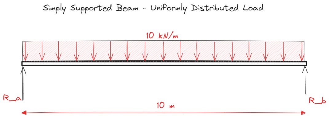
Today, we are jumping straight into a simple engineering example to solve a simply supported beam subjected to a uniformly distributed load (UDL). This is fundamental from an engineering perspective but demonstrates many of the great features of Python.

Learning through practical examples, particularly those rooted in familiar engineering concepts, offers an intuitive pathway to grasp the versatility of Python.

While the underlying principles of beam theory may be familiar to many engineers, applying Python to solve these problems introduces a novel and efficient method to analyze and visualize this simply supported beam. If you have yet to dig into Python syntax, it may appear strange or complex, but run through it and see how you feel. Don’t be concerned if you feel confused. It takes some time to piece it together, and we will.

This example provides:

Contextualized Understanding: Applying Python to well-understood engineering problems allows engineers to see immediate applications of programming concepts, in this case, procedural programming. Code is executed line by line in a defined sequence, just as you would solve this problem with a pencil, Excel, or whatever tool you use.
Enhanced Problem-Solving Skills: You will see some mathematical expressions in the code snippets that define the plots. There are interesting tricks and perspectives to gain from this aspect of Python that have helped reframe the way I think about certain numerical problems.
Immediate Feedback Loop: Visualizing the impact of different loads and lengths on beam behaviour through plotting provides instant feedback, crucial for refining understanding, testing sensitivities and debugging code.
Bridging Theory and Practice: This approach closes the gap between theoretical knowledge and practical application, showing how abstract concepts are used in tangible scenarios.

Acknowledging the Learning Curve

It's important to recognize that this example, while designed to be accessible, touches on numerous concepts that extend beyond the immediate grasp of beginners in Python. These include:

Python Syntax and Constructs: Variables, functions, and loops are foundational to programming but do require time to master.
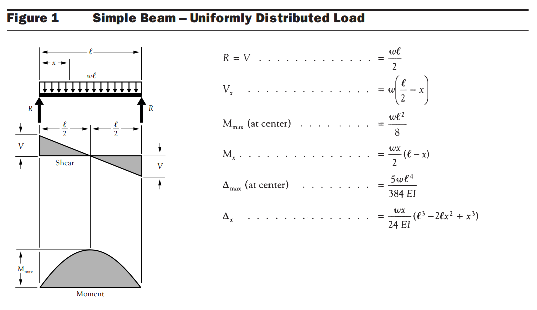
Use of Libraries: Utilizing numpy and matplotlib introduces the concept of libraries, which are external codebases that extend Python's functionality. Libraries are the key to the true flexibility of Python.
Engineering Concepts: The principles of shear forces and bending moments, though familiar to engineers, are combined with programming, potentially complicating their understanding, especially if you haven’t solved any beams like this in a while! But don’t worry; this sample is from the good old NDS Beam Formula Design Aid No. 6.
NDS Beam Formula Design Aid No. 6
Plotting and Visualization: Graphically representing data requires understanding the mathematical concepts behind the data and the technical details of plot customization. Plotting is the most complex but useful aspect.

There’s a Brazilian expression my friend uses that fits the bill.

“Sometimes, we have to cook the fish and watch the cat.” - Thomas Lisboa

This means that to do something complex, we often need to do many things in unison, and none of them easy.

Recommended Prerequisites

To fully benefit from this example, a baseline familiarity with the following areas is advantageous but not required:

Basic Programming Concepts: Understanding variables, loops, and functions in any programming language.
Fundamental Python Knowledge: A grasp of Python syntax and the ability to write simple scripts.
Engineering Fundamentals: Basic knowledge of statics and mechanics of materials, including beam theory and load effects.

Flocode Courses: A Deeper Dive

Recognizing the breadth of concepts introduced, the Flocode Essentials course is designed to break down these elements into manageable, digestible pieces. Starting from the very basics of Python programming, the courses will guide learners through:

Step-by-Step Python Syntax Exploration: Building a solid foundation in Python essentials before tackling complex problems.
Application of Python in Engineering: Demonstrating how Python can be used to automate calculations, analyze data, and solve real-world engineering problems.
In-depth Analysis of Engineering Concepts: Providing a refresher on engineering principles as they are applied, ensuring a comprehensive understanding of both the engineering challenges and the Python solutions.
Intro to Plotting Techniques: Delving into data visualization, showing how to create more sophisticated and informative plots.

By covering these topics in detail, we aim to equip engineers with the skills they need to integrate Python into their professional toolkit, enhancing their capabilities and efficiency. This practical example is just a small step at the beginning of a journey to unlock the full potential of Python in engineering, ensuring learners are not just coding but innovating in a way that works for them.

Sign up for the waitlist. Flocode’s Beta Program is coming soon for a smaller group. I’ll notify subscribers about this as soon as we are ready to start testing.

A Simply Supported Beam

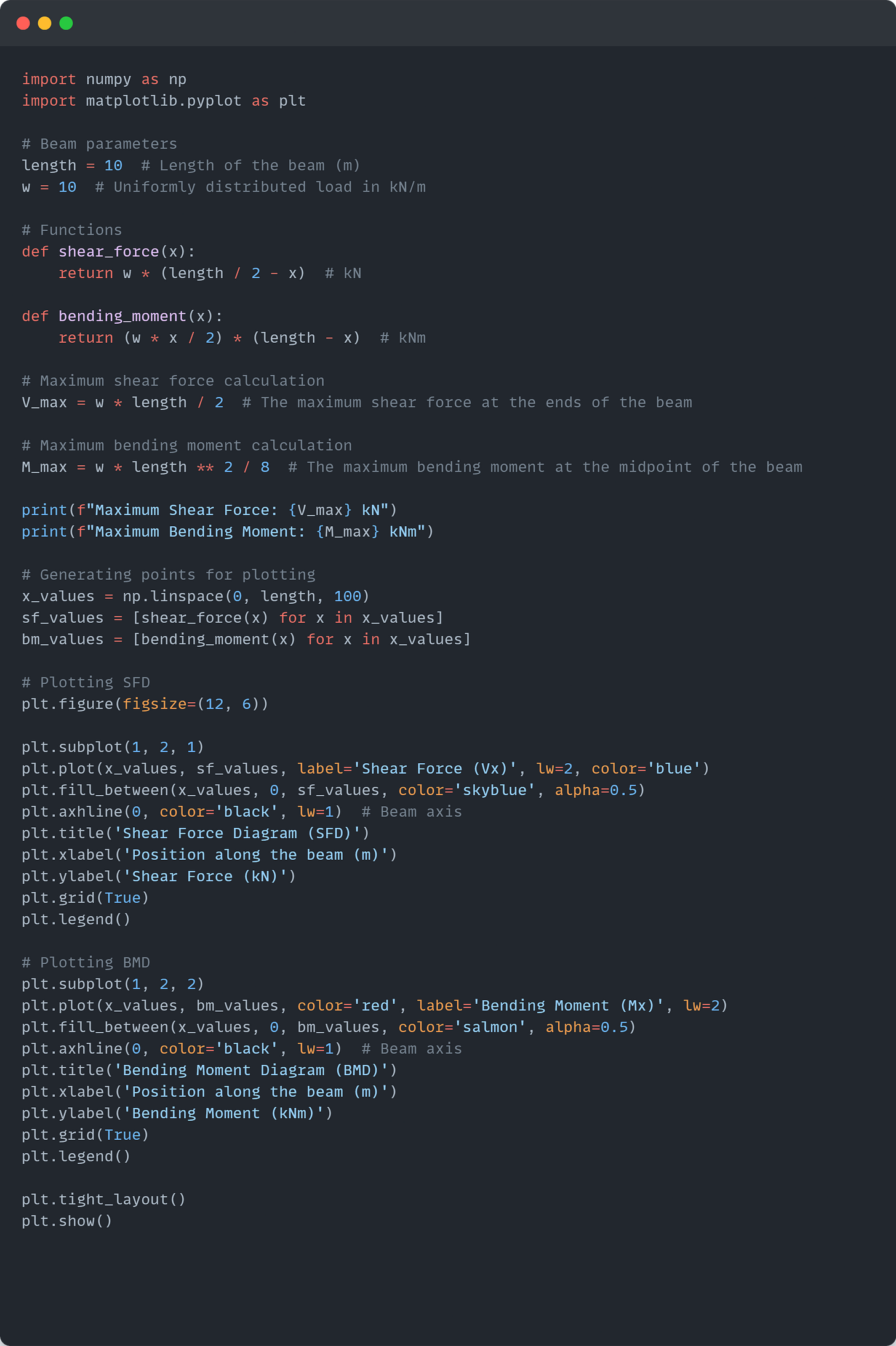
Firstly, the code is available in a GitHub Gist if you want to copy it and play around. You can't copy the code from the image below, but it does show Python syntax highlighting. Substack is still figuring out its disgraceful code syntax presentation. I thought the image be easier on your eyeballs.

Take a first glance at the code below, read through it, and then we will walk through what is happening.

Outputs

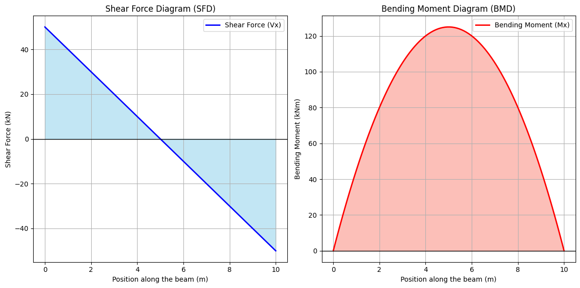
Once we run the code, the following outputs, our results and plots, are produced.

Maximum Shear Force: 50.0 kN
Maximum Bending Moment: 125.0 kNm

Code Walkthrough

Again, there are many things happening in this example but the intent is to show you a familiar situation so you can calibrate yourself with what's involved.

I will cover this in much more detail in Flocode’s courses. But there's enough ammo here for you to begin experimenting with other engineering formulas in a similar fashion.

Step 0: Import the Libraries

I usually work in a Jupyter Notebook; once we've set one up, we need to import our required libraries, NumPy and Matplotlib. These are two absolutely essential libraries for scientific computing.

You can read about Jupyter Notebooks in a previous article here:

#013 - Python Essentials | 01 - Jupyter Notebooks Part 1/3

import numpy as np
import matplotlib.pyplot as plt

Step 1: Define Beam Parameters

length = 10  # Length of the beam (m)
w = 10  # Uniformly distributed load in kN/m

These lines of code set the foundational parameters: the beam's length and the magnitude of its load. This code defines variables (length, w) and tells the readers about the units through comments ( text preceded by a ‘#’). Comments are incredibly useful and do not affect the code; they are used purely to describe what’s happening for the code creator/reviewer. Comments are essential to keep track of your thoughts and logic.

Step 2: Function Definitions

def shear_force(x):
    return w * (length / 2 - x)  # kN

def bending_moment(x):
    return (w * x / 2) * (length - x)  # kNm

We define functions to calculate the shear force and bending moment at any point x along the beam, incorporating basic beam theory.

Interestingly, you can see ‘def’ and ‘return’ highlighted in a different colour; that’s because these are keywords that perform specific actions within the Python syntax, ‘def’ meaning ‘define’ and ‘return’ meaning that it exits a function and optionally passes a value.

What’s a function? We’ll talk about that another day, despite the fact that they are outrageously important.

Step 3: Maximum Values Calculation

V_max = w * length / 2  # Maximum shear force
M_max = w * length ** 2 / 8  # Maximum bending moment

Calculates our maximum shear force and bending moment.

Note that ‘**’ is an exponent operator, just like ‘^’ in Excel or MathCad.

Step 4: Generating Points for Plotting

This is where things get a little more abstract, especially if you’re coming from Excel.

x_values = np.linspace(0, length, 100)

This NumPy method generates a series of points along the beam, between 2 points (0 and ‘length’), to evaluate the shear force and bending moment. The ‘100’ means that the line is divided into 100 equal segments to give us a smooth curve.

Step 5: Plotting Diagrams

The plotting is done in two main parts, using matplotlib:

Shear Force Diagram (SFD)
Bending Moment Diagram (BMD)

plt.figure(figsize=(12, 6))

Sets up the plotting environment, defining the figure size (12 inches by 6 inches).

SFD Plotting

plt.subplot(1, 2, 1)
plt.plot(x_values, sf_values, label='Shear Force (Vx)', lw=2, color='blue')
plt.fill_between(x_values, 0, sf_values, color='skyblue', alpha=0.5)
plt.axhline(0, color='black', lw=1)  # Beam axis

Each line of the code has a specific role in creating the visual representation of the shear forces along the beam. Let's break down each part of the code for clarity:

plt.subplot(1, 2, 1) is a function call that creates a subplot in a figure. The arguments (1, 2, 1) define the subplot's layout and position. Here, 1, 2 means that the figure is divided into 1 row and 2 columns, effectively creating a space for two plots side by side. The last 1 specifies that the following plotting commands will be applied to the first subplot. This is where the shear force diagram will be plotted.
plt.plot(x_values, sf_values, ...) plots the shear force values (sf_values) against positions along the beam (x_values). The label parameter is used to identify the plotted data in the legend with 'Shear Force (Vx)'. The lw=2 sets the line width to 2, making the plot line thicker for better visibility, and color='blue' specifies the line’s colour.
plt.fill_between(...) fills the area between the plot line and the x-axis. This function takes the same x_values for the horizontal axis and fills the area between 0 (the baseline) and sf_values (the shear force values). The color='skyblue' and alpha=0.5 parameters set the fill colour and make it semi-transparent (alpha controls the opacity, where 0 is fully transparent and 1 is fully opaque), respectively. This visual enhancement helps emphasize the shear force distribution along the beam.
plt.axhline(0, ...) draws a horizontal line (axis line) across the plot at y=0, which represents the beam axis in this context. The color='black' and lw=1 parameters define this axis line's colour and width, making it a reference point that visually anchors the plot, indicating the beam's neutral axis where shear forces change from positive to negative or vice versa.

Together, these commands create a detailed visual representation of the shear force distribution along a beam, highlighting the magnitude and direction of shear forces at different points. There are more straightforward and more complicated ways to do this, with varying levels of depth and complexity. The strength of good visuals for engineering design can not be overstated, both for your personal understanding of your work and for the effective communication of it.

BMD Plotting

plt.subplot(1, 2, 2)
plt.plot(x_values, bm_values, color='red', label='Bending Moment (Mx)', lw=2)
plt.fill_between(x_values, 0, bm_values, color='salmon', alpha=0.5)
plt.axhline(0, color='black', lw=1)  # Beam axis

Illustrates bending moments, similarly enhanced with shading.

Step 6: Axis and Labels

Each plot is labelled with titles, axis labels, and grids for clarity.

plt.title('Shear Force Diagram (SFD)')
plt.xlabel('Position along the beam (m)')
plt.ylabel('Shear Force (kN)')
plt.grid(True)
plt.legend()

Adds informative labels and a legend to the plot.

Note that ‘True’ is what we refer to as a ‘Boolean’ in Python. It represents one of the two values in Boolean logic. The other value is ‘False’ 😱.

Booleans are used in programming to perform logical operations like comparisons and conditions, leading to control flow decisions within the code. Very useful stuff.

Conclusion

It might feel like there’s a lot to digest, but once you do it once, it’s easy to wrap the entire process in a single-line function; consider something like this;

plot_simply_supported_beam_diagrams(length=10, w=10)

This function, plot_simply_supported_beam_diagrams can encapsulate the entire process of calculating and plotting the shear force and bending moment diagrams. By calling this function with different values for length and w, you can easily generate diagrams for various beams and loading conditions without repeating the code.

Similarly, you can loop through a list of beams of different lengths or loads. Imagine how easy it is to apply your code to many different situations very quickly.

This example is intended to give you a broad conceptual overview of one simple application of Python for engineers.

Give me feedback or requests for the type of content you are interested in; the possibilities are endless. Some ideas…

Thank you once more for your time and attention. If you want to join the Beta Program, remember to sign up on the Flocode Waitlist. I’m incredibly excited to start speaking to some of you to discover your goals and engineering backgrounds as we build the community platform.

Flocode has members in 84 countries around the world. China, Kazakhstan, and Greenland. ESPECIALLY GREENLAND, we’re coming for you! And Mexico, don’t think we don’t see you! I’m only having a laugh. I'm incredibly grateful for the support and good wishes, wherever you are (except Greenland).

Take care of yourself, and keep innovating.

See you in the next one.

James 🌊